GeeraerdST inactivation model for microbial inactivation curve.
Returns the model parameters estimated according to data collected in microbial inactivation experiments.
Arguments
- x
is a numeric vector indicating the heating time under a constant temperature of the experiment
- Y0
is the initial (time=0) bacterial concentration (ln(N0))
- Yres
is a low asymptote reflecting the presence of a resistant sub-population (ln(Nres))
- kmax
is the maximum inactivation rate
- Sl
represents shoulder phase preceding the sharp inactivation slope of the curve
Details
The model's inputs are:
t: time, assuming time zero as the beginning of the experiment.
N(t): the bacterial concentration measured at time t.
Users should make sure that the bacterial concentration input is entered
in natural logarithm, Y(t) = ln(N(t)).
References
Geeraerd AH, Valdramidis VP, Van Impe JF (2005). “GInaFiT, a freeware tool to assess non-log-linear microbial survivor curves.” International Journal of Food Microbiology, 102(1), 95-105. ISSN 0168-1605, doi:10.1016/j.ijfoodmicro.2004.11.038 .
Author
Vasco Cadavez vcadavez@ipb.pt and Ursula Gonzales-Barron ubarron@ipb.pt
Examples
library(gslnls)
data(mafart2005Li11)
mafart2005Li11$lnN <- log(10) * mafart2005Li11$logN
initial_values <- list(Y0 = 18, Yres = 2, kmax = 0.7, Sl = 4)
fit <- gsl_nls(lnN ~ GeeraerdST(Time, Y0, Yres, kmax, Sl),
data = mafart2005Li11,
start = initial_values
)
summary(fit)
#>
#> Formula: lnN ~ GeeraerdST(Time, Y0, Yres, kmax, Sl)
#>
#> Parameters:
#> Estimate Std. Error t value Pr(>|t|)
#> Y0 23.19298 0.19490 119.000 2.37e-11 ***
#> Yres 15.96547 0.18039 88.504 1.40e-10 ***
#> kmax 0.59485 0.05436 10.943 3.46e-05 ***
#> Sl 5.67219 0.82123 6.907 0.000455 ***
#> ---
#> Signif. codes: 0 ‘***’ 0.001 ‘**’ 0.01 ‘*’ 0.05 ‘.’ 0.1 ‘ ’ 1
#>
#> Residual standard error: 0.2744 on 6 degrees of freedom
#>
#> Number of iterations to convergence: 12
#> Achieved convergence tolerance: 8.882e-16
#>
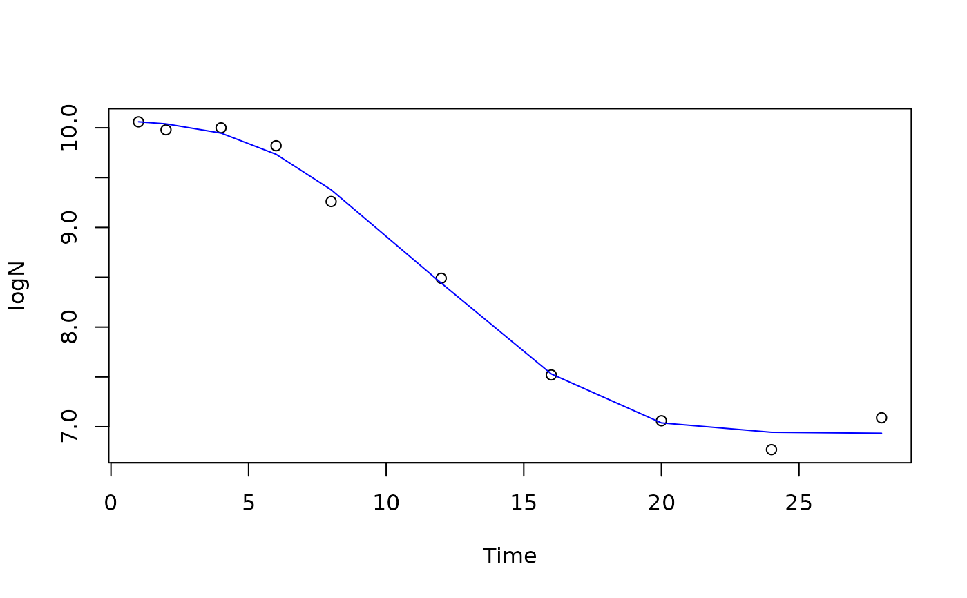
plot(lnN ~ Time, data = mafart2005Li11)
lines(mafart2005Li11$Time, predict(fit), col = "blue")