Huang full growth model

HuangFM function to fit the Huang full growth model to complete microbial growth curve. Returns the model parameters estimated according to data collected in microbial growth experiments.

Usage

HuangFM(t, Y0, Ymax, MUmax, lag)

Arguments

t

is a numeric vector indicating the time of the experiment

Y0

is the natural logarithm of the initial microbial concentration (ln(N0)) at time=0

Ymax

is the natural logarithm of the maximum concentration (ln(Nmax)) reached by the microorganism

MUmax

is the maximum specific growth rate given in time units

lag

is the duration of the lag phase in time units

Value

An object of nls class

Details

Model's inputs are:

t: time, assuming time zero as the beginning of the experiment.

Y(t): the natural logarithm of the microbial concentration (ln(N(t)) measured at time t.

Users should make sure that the microbial concentration input is entered in natural logarithm, Y(t) = ln(X(t)).

References

Huang L (2008). “Growth Kinetics of Listeria monocytogenes in Broth and Beef Frankfurters-Determination of Lag Phase Duration and Exponential Growth Rate under Isothermal Conditions.” Journal of Food Science, 73(5), E235-E242. doi:10.1111/j.1750-3841.2008.00785.x .

Author

Vasco Cadavez, vcadavez@ipb.pt and Ursula Gonzales-Barron, ubarron@ipb.pt

Examples

## Example: Huang full model
library(gslnls)
data(growthfull)  # simulated data set.
initial_values = list(Y0=0, Ymax=22, MUmax=1.7, lag=5) # define the initial values
## Call the fitting function
fit <- gsl_nls(lnN ~ HuangFM(Time, Y0, Ymax, MUmax, lag),
           data=growthfull,
           start =  initial_values)
summary(fit)
#> 
#> Formula: lnN ~ HuangFM(Time, Y0, Ymax, MUmax, lag)
#> 
#> Parameters:
#>       Estimate Std. Error t value Pr(>|t|)    
#> Y0     0.04562    0.25768   0.177    0.863    
#> Ymax  21.13232    0.22393  94.372 8.54e-15 ***
#> MUmax  1.85942    0.06076  30.601 2.08e-10 ***
#> lag    5.07987    0.25000  20.320 7.89e-09 ***
#> ---
#> Signif. codes:  0 ‘***’ 0.001 ‘**’ 0.01 ‘*’ 0.05 ‘.’ 0.1 ‘ ’ 1
#> 
#> Residual standard error: 0.4444 on 9 degrees of freedom
#> 
#> Number of iterations to convergence: 5 
#> Achieved convergence tolerance: 9.033e-13
#> 

confint(fit)
#>        2.5 %     97.5 %
#> 1 -0.5372874  0.6285347
#> 2 20.6257592 21.6388712
#> 3  1.7219672  1.9968814
#> 4  4.5143280  5.6454030

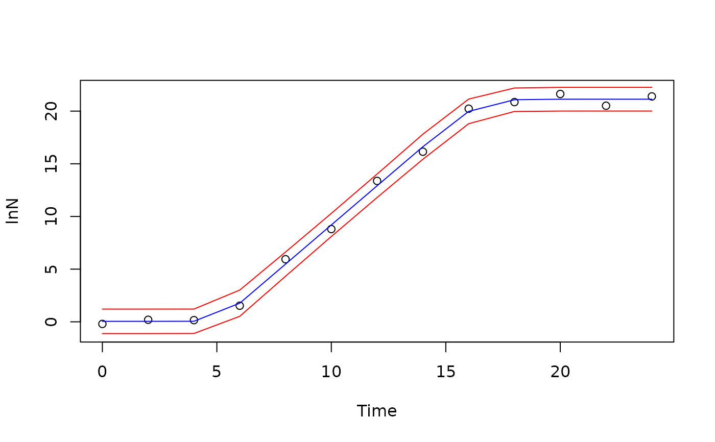
preds <- data.frame(predict(fit, interval = "prediction", level = 0.95))
plot(lnN ~ Time, data=growthfull, ylim=c(-1,22))
lines(growthfull$Time, preds$fit, col="blue")
lines(growthfull$Time, preds$upr, col="red")
lines(growthfull$Time, preds$lwr, col="red")