Weibull inactivation model Mafart

WeibullM inactivation model for microbial inactivation curve. Returns the model parameters estimated according to data collected in microbial inactivation experiments.

Usage

WeibullM(x, Y0, sigma, alpha)

Arguments

x

is a numeric vector indicating the heating time under a constant temperature of the experiment

Y0

is the natural logarithm of the initial (time=0) bacterial concentration (N0)

sigma

is the time of first decimal reduction

alpha

which is a shape parameter

Value

A numeric vector with the fitted values

Details

The model's inputs are:

t: time, assuming time zero as the beginning of the experiment.

Y(t): the natural logarithm of the bacterial concentration (ln(N(t))) measured at time t.

Users should make sure that the bacterial concentration input is entered in natural logarithm, Y(t) = ln(N(t)).

References

Mafart P, Couvert O, Gaillard S, Leguerinel (2002). “On calculating sterility in thermal preservation methods: application of the Weibull frequency distribution model.” International Journal of Food Microbiology, 72, 107-113.

Author

Vasco Cadavez vcadavez@ipb.pt and Ursula Gonzales-Barron ubarron@ipb.pt

Examples

library(gslnls)
data(bixina)
initial_values <- list(Y0 = 5.75, sigma = 12.8, alpha = 2.4)
fit <- gsl_nls(lnN ~ WeibullM(Time, Y0, sigma, alpha),
  data = bixina,
  start = initial_values
)
summary(fit)
#> 
#> Formula: lnN ~ WeibullM(Time, Y0, sigma, alpha)
#> 
#> Parameters:
#>       Estimate Std. Error t value Pr(>|t|)    
#> Y0     5.53341    0.03894  142.09  < 2e-16 ***
#> sigma 12.87224    0.13543   95.05  < 2e-16 ***
#> alpha  2.39535    0.13162   18.20 1.23e-11 ***
#> ---
#> Signif. codes:  0 ‘***’ 0.001 ‘**’ 0.01 ‘*’ 0.05 ‘.’ 0.1 ‘ ’ 1
#> 
#> Residual standard error: 0.09671 on 15 degrees of freedom
#> 
#> Number of iterations to convergence: 4 
#> Achieved convergence tolerance: 6.106e-16
#> 

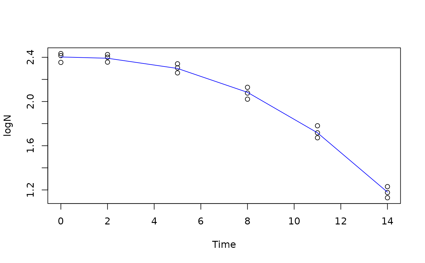
plot(lnN ~ Time, data = bixina)
lines(bixina$Time, predict(fit), col = "blue")