Weibull inactivation model Peleg and Huang

WeibullPH inactivation model for microbial inactivation curve. Returns the model parameters estimated according to data collected in microbial inactivation experiments.

Usage

WeibullPH(t, Y0, k, alpha)

Arguments

t: is a numeric vector indicating the time of the experiment
Y0: is the natural logarithm of the initial (time=0) bacterial concentration
k: is the inactivation rate (ln units/time)
alpha: is the shape parameter

Value

A numeric vector with the fitted values

Details

The model's inputs are:

t: time, assuming time zero as the beginning of the experiment.

Y(t): the natural logarithm of the bacterial concentration X(t) measured at time t.

Users should make sure that the bacterial concentration input is entered in natural logarithm, Y(t) = ln(X(t)).

The following parameters can be estimated using Weibull function:

t: is heating time under a constant temperature

Y0: is the initial (time=0) bacterial counts in natural logarithm of the initial bacterial counts;

k: is the inactivation rate (ln units/time)

alpha: is the shape parameter of the survival curve

References

Huang L (2009). “Thermal inactivation of Listeria monocytogenes in ground beef under isothermal and dynamic temperature conditions.” Journal of Food Engineering, 90(3), 380-387. ISSN 0260-8774, doi:10.1016/j.jfoodeng.2008.07.011 .

Author

Vasco Cadavez vcadavez@ipb.pt and Ursula Gonzales-Barron ubarron@ipb.pt

Examples

library(gslnls)
data(bixina)
initial_values <- list(Y0 = 6.0, k = 1.0, alpha = 0.2)
fit <- gsl_nls(lnN ~ WeibullPH(Time, Y0, k, alpha),
  data = bixina,
  start = initial_values
)
summary(fit)
#> 
#> Formula: lnN ~ WeibullPH(Time, Y0, k, alpha)
#> 
#> Parameters:
#>        Estimate Std. Error t value Pr(>|t|)    
#> Y0    5.5334088  0.0389420  142.09  < 2e-16 ***
#> k     0.0021978  0.0007657    2.87   0.0117 *  
#> alpha 2.3953478  0.1316153   18.20 1.23e-11 ***
#> ---
#> Signif. codes:  0 ‘***’ 0.001 ‘**’ 0.01 ‘*’ 0.05 ‘.’ 0.1 ‘ ’ 1
#> 
#> Residual standard error: 0.09671 on 15 degrees of freedom
#> 
#> Number of iterations to convergence: 29 
#> Achieved convergence tolerance: 0
#> 

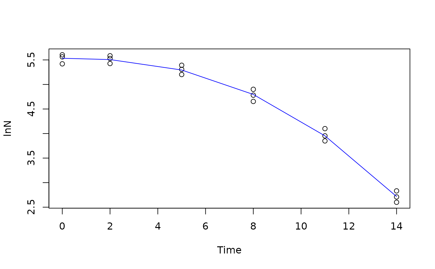
plot(lnN ~ Time, data = bixina)
lines(bixina$Time, predict(fit), col = "blue")